Approximate Recovery in Near-linear Time by Forest Pursuit

“Does the pursuit of truth give you as much pleasure as before? Surely it is not the knowing but the learning, not the possessing but the acquiring, not the being-there but the getting there that afford the greatest satisfaction.”

– Carl Friedrich Gauss

In this chapter, we build on the notion of “Desire Path” estimation of a dependency network from node activations — sampling from a class of subgraphs constrained to active nodes, then merging them. We present Forest Pursuit (FP), a method that is scalable, trivially parallelizes, and offline-capable, while also outperforming commonly used algorithms across a battery of standardized tests and metrics. The key application for using FP is in domains where node activation can be reasonably modeled as arising due to random walks—or similar spreading process—on an underlying dependency graph.

Because we wish to model our node activations as being caused by other nodes (that they depend on), we draw a connection to a class of models for spreading, or, diffusive processes. We outline how random-walks are related to these diffusive models of graph traversal, enabled by an investigation of the graph’s “regularized laplacian” from [1].

First, we build an intuition for the use of trees as an unbiased estimator for desire path estimation when spreading processes are at work on the latent network. Then, the groundwork for FP is laid by combining sparse approximation through matching pursuit with a loss function modeled after the Chow Liu representation for joint probability distributions. The approximate complexity for FP is linear in the spreading rate of the modeled random walks, and linear in dataset size, while running in $O(1)$ time with respect to the network size. This departs dramatically from other methods in the space, all of scale in the number of nodes in the entire network. We then test FP against an array of alternative methods (including GLASSO) with MENDR, our proposed standard reference dataset and testbench for network recovery. FP outperforms other tested algorithms in nearly every case, and empirically confirms its complexity scaling for sub-thousand network sizes.

Random Walks as Spanning Forests

The class of diffusive processes we focus on “spread” from one node to another. If a node is activated, it is able to activate other nodes it is connected to, directly encoding our need for the graph edges to represent that nodes “depend” on others to be activated. In this case, a node activates when another node it depends on spreads their state to it. These single-cause activations are often modeled as a random-walk on the dependency graph: visiting a node leads to its activation.

Random Walk Activations

Random walks are regularly employed to model spreading and diffusive processes on networks. If a network consists of locations, states, agents, etc. as “nodes”, and relationships between nodes as “edges”, then random walks consist of a stochastic process that “visits” nodes by randomly “walking” between them along connecting edges. Epidemiological models, cognitive search in semantic networks, website traffic routing, social and information cascades, and many other domains also involving complex systems, have used the statistical framework of random walks to describe, alter, and predict their behaviors. [2], [3], [4], [5], [6]

[2]

S. Kim, J. Breen, E. Dudkina, F. Poloni, and E. Crisostomi, “On the effectiveness of random walks for modeling epidemics on networks,” PLOS ONE, vol. 18, no. 1, p. e0280277, Jan. 2023, doi: 10.1371/journal.pone.0280277.

[4]

K.-S. Jun, J. Zhu, T. T. Rogers, Z. Yang, et al., “Human memory search as initial-visit emitting random walk,” Advances in neural information processing systems, vol. 28, no. 20, pp. 2389–2393, 2015, doi: 10.1016/j.physleta.2019.04.060.

[5]

P. G. Doyle and J. L. Snell, “Random walks and electric networks.” arXiv, 2000. doi: 10.48550/ARXIV.MATH/0001057.

[6]

M. Mane, D. DeLaurentis, and A. Frazho, “A markov perspective on development interdependencies in networks of systems,” Journal of Mechanical Design, vol. 133, no. 10, Oct. 2011, doi: 10.1115/1.4004975.

[7]

B. Rozemberczki, O. Kiss, and R. Sarkar, “Little ball of fur: A python library for graph sampling,” 2020, doi: 10.48550/ARXIV.2006.04311.

[8]

M. E. J. Newman, “The structure and function of complex networks,” SIAM Review, vol. 45, no. 2, pp. 167–256, Jan. 2003, doi: 10.1137/s003614450342480.

¹ For a brief treatment of the case that INVITE emission order is preserved, see Recovery from Working Memory & Partial Orders

When network structure is known, the dynamics of random-walks are used to capture the network structure via sampling [7], estimate node importance’s[Mathematicsnetworks_Newman2018], or predict phase-changes in node states (e.g., infected vs. uninfected)[8]. In our case, since we have been encoding the activations as binary activation vectors, the “jump” information is lost—activations are “emitted” for observation only upon the random walker’s initial visit.[4] Further, the ordering of emissions has been removed in our binary vector representation, leaving only co-occurrence groups in each $\mathbf{x}_i$.¹ In many cases, however, the existence of relationships is not known already, and analysts might assume their data was generated by random-walk-like processes, and want to use that knowledge to estimate the underlying structure of the relationships between nodes.

Activations in a Forest

As a general setting, the number of node activations (e.g., for datasets like co-authorship) is much smaller than the set of nodes ($\|\mathbf{x}_i\in\mathbb{S}^n\|_0 \ll n$)²
[1] go to some length describing discrete- and continuous-time random walk models that can give rise to binary activation vectors like our $X(i,j):I\times J\rightarrow \mathbb{B}$. The regularized laplacian (or forest) kernel of a graph[9] plays a central role in their analysis, as it will in our discussion going forward.

² $\|\cdot\|_0$ is the $\ell_0$ “pseudonorm”, counting non-zero elements (the support) of its argument.

[9]

K. Avrachenkov, P. Chebotarev, and D. Rubanov, “Similarities on graphs: Kernels versus proximity measures,” European Journal of Combinatorics, vol. 80, pp. 47–56, Aug. 2019, doi: 10.1016/j.ejc.2018.02.002.

\[ Q_{\beta} = (I+\beta L)^{-1} \tag{6.1}\]

In that work, it is discussed as the optimal solution to the semi-supervised “node labeling” problem, having a regularization parameter $\beta$, though its uses go far beyond this.[10], [11], [12] $Q$ generalizes the so-called “heat kernel” $\exp{(-t\tilde{L})}$, in the sense that it solves a lagrangian relaxation of a loss function based on the heat equation. This can be related to the PageRank ($\exp{(-tL_{\text{rw}})}$) kernel as well, which is explicitly based on random walk transition probabilities.

[10]

J. Pang and G. Cheung, “Graph laplacian regularization for image denoising: Analysis in the continuous domain,” IEEE Transactions on Image Processing, vol. 26, no. 4, pp. 1770–1785, Apr. 2017, doi: 10.1109/TIP.2017.2651400.

[11]

O. Knill, “Counting rooted forests in a network,” arXiv, arXiv:1307.3810, Jul. 2013. doi: 10.48550/arXiv.1307.3810.

[12]

P. Chebotarev and E. Shamis, “The matrix-forest theorem and measuring relations in small social groups,” arXiv, arXiv:math/0602070, Feb. 2006. doi: 10.48550/arXiv.math/0602070.

³ $Q$ can also be interpreted as a continuous-time random walk location probability, after exponentially distributed time, if spending exponentially-distributed time in each node.

⁴ edge weights scaled by

In fact, $Q$ can be viewed as a transition matrix for a random walk having a geometrically distributed number of steps, giving us a small expected support for $\mathbf{x}_i$, as needed.³ However we interpret $Q$, a remarkable fact emerges due to a theorem by Chebotarev[11], [12]: each entry $q=Q(u,v)$ is equal to the probability⁴ that nodes $u,v$ are connected in a randomly sampled spanning rooted forest

In other words, co-occurring node activations due to a random walk or heat kernel are deeply tied to the chance that those nodes find themselves on the same tree in a forest.

Spreading Dependencies as Trees

With the overt link from spreading processes to counts of trees made, there’s room for a more intuitive bridge.

For single-cause, single source spreading process activations—on a graph—the activation dependency graph for each observation/spread/random walk must be a tree. With a single cause (the “root”), which is the starting position of a random walker, a node can only be reached (activated) by another currently activated node. If the random walk jumps from one visited node to another, previously visited one, that transition did not result in an activation, so the dependency count for that edge should not increase. This description of a random walk, where subsequent visits do not “store” the incoming transition, is roughly equivalent to one more commonly described as a Loop-Erased random walk. It is precisely used to uniformly sample the space of spanning trees on a graph.[13]

[13]

D. B. Wilson, “Generating random spanning trees more quickly than the cover time,” in Proceedings of the twenty-eighth annual ACM symposium on theory of computing - STOC ’96, in STOC ’96. ACM Press, 1996, pp. 296–303. doi: 10.1145/237814.237880.

Much like a reluctant co-author “worn down” by multiple collaboration requests, we can even include random walks that “receive” activation potential from more than one source. Say a node is activated when some fraction of its neighbors have all originated a random walk transition to it, or a node activates on its second visit, or similar. We simply count (as dependency evidence) the ultimate transition that precipitated activation. This could be justified from an empirical perspective as well: say we observe an author turn down requests for one paper from two individuals, but accept a third. We could actually infer a lowered dependency on the first two, despite the eventual coauthorship. Only the interaction that was observed as successful necessarily counts toward success-dependency, barring any contradicting information.

It’s important to add here that mutual convincing by multiple collaborators simultaneously (or over time) is expressly left out. In other words, only pairwise interactions are permitted. This is not an additional assumption, but a key limitation of our use of graphs in the first place! As Torres et al. go to great lengths elaborating in [14], it is critical to correctly model dependencies when selecting a structural representation of our problem to avoid data loss. The possibility for multi-way interactions would necessitate the use of either a simplicial complex or a hypergraph as the carrier structure, not a graph.

[14]

L. Torres, A. S. Blevins, D. Bassett, and T. Eliassi-Rad, “The why, how, and when of representations for complex systems,” SIAM Rev., vol. 63, no. 3, pp. 435–485, Jan. 2021, doi: 10.1137/20M1355896.

Figure 6.1: Edge Measurements with true (tree) dependencies known

Figure 6.1 demonstrates the use of trees as the distribution for subgraphs, instead of outer-products/cliques.

Sparse Approximation

As indicated previously, we desire a representation of each observation that takes the “node space” vectors ($\mathbf{x}_i$) to “edge space” ones ($\mathbf{r}_i$). We have separated each observation with the intention of finding a point-estimate for the “best” edges, such that the edge vector induces a subgraph belonging to a desired class. If we assume that each edge vector is in $\mathbb{B}^{\omega}$, so that the interactions are unweighted, undirected, simple graphs, then for any family of subgraphs we will be selecting from at most $\omega\leq {n\choose 2}$ edges.

Representing a vector as a sparse combination of a known set of vectors (also known as “atoms”) is called sparse approximation.

Problem Specification

Sparse approximation of a vector $\mathbf{x}$ as a representation $\mathbf{r}$ using a dictionary of atoms (columns of $D$) is specified more concretely as [15]: \[\mathbf{\hat{r}} = \operatorname*{argmin}_{\mathbf{r}}{\|\mathbf{x}-D\mathbf{r} \|_2^2} \quad \text{s.t.} \|\mathbf{r}\|_0\leq N \tag{6.2}\] where $N$ serves as a sparsity constraint (at most $N$ non-zero entries). This is known to be NP-hard, though a number of efficient methods to approximate a solution are well-studies and widely used. Solving the Lagrangian form of Equation 6.2, with an $\ell_1$-norm in place of $\ell_0$, is known as Basis Pursuit[16], while greedily solving for the non-zeros of $\mathbf{r}$ one-at-a-time is called matching pursuit[17]. In that work, each iteration selects the atom with the largest inner product $\langle \mathbf{d}_{i'},\mathbf{x}\rangle$.

[15]

R. Rubinstein, M. Zibulevsky, and M. Elad, “Efficient implementation of the k-SVD algorithm using batch orthogonal matching pursuit,” Cs Technion, vol. 40, no. 8, pp. 1–15, 2008.

[16]

B. K. Natarajan, “Sparse approximate solutions to linear systems,” SIAM Journal on Computing, vol. 24, no. 2, pp. 227–234, Apr. 1995, doi: 10.1137/s0097539792240406.

[17]

S. G. Mallat and Z. Zhang, “Matching pursuits with time-frequency dictionaries,” IEEE Transactions on Signal Processing, vol. 41, no. 12, pp. 3397–3415, 1993, doi: 10.1109/78.258082.

We take an approach similar to this, but with the insight that the inner product will not result in desired sparsity (namely, a tree). Our dictionary in this case will be the set of edges given by $B$ (see Subgraph Distributions), while our sparsity is given by the relationship of the numbers of nodes and edges in a tree: \[ \mathbf{\hat{r}} = \operatorname*{argmin}_{\mathbf{r}}{\|\mathbf{x}-B^T\mathbf{r} \|_2^2} \quad \text{s.t.}\quad \|\mathbf{r}\|_0 = \|\mathbf{x}\|_0 - 1 \tag{6.3}\]

There are some oddities to take into account here. As a linear operator (see Models & linear operators), $B^T$ takes a vector of edges to node-space, counting the number of edges each node was incident to. This means that, even with a ground-truth set of interactions, $B^T$ would take them to a new matrix $X_{\text{deg}}(i,j):I\times J \rightarrow \mathbb{N}$, which has entries of the number of interactions each individual in observation $i$ was involved in. While very useful for downstream analysis (see Forest Pursuit as Preprocessing), the MSE loss in Equation 6.4 will never be zero, since $X_{\text{deg}}$ entries are not boolean. Large-degree “hub” nodes in the true graph would give a large residual, and the adjoint would subsequently fail to remove the effect of $B^T$ on the edge vectors.

It might be possible to utilize a specific semiring, such as $(\min,+)$, to enforce inner products (see Distance vs. Incidence) that take us back to a binary vector. This would be more than a simple hack, and belies a great depth of possible connection to the problem at hand. It is known that “lines” (arising from equations of the inner product) in tropical projective space are trees.[18] In addition, the tropical equivalent to Kirchoff’s polynomial (which counts over all possible spanning trees), is the direct computation of the minimum spanning tree.[19] For treatment of sparse approximation using tropical matrix factorization, see [20]

[18]

“The tropical grassmannian,” advg, vol. 4, no. 3, pp. 389–411, Jul. 2004, doi: 10.1515/advg.2004.023.

[19]

S. Jukna and H. Seiwert, “Tropical kirchhoff’s formula and postoptimality in matroid optimization,” Discrete Applied Mathematics, vol. 289, pp. 12–21, Jan. 2021, doi: 10.1016/j.dam.2020.09.018.

[20]

A. Omanović, H. Kazan, P. Oblak, and T. Curk, “Sparse data embedding and prediction by tropical matrix factorization,” BMC Bioinformatics, vol. 22, no. 1, Feb. 2021, doi: 10.1186/s12859-021-04023-9.

[21]

D. P. Wipf and B. D. Rao, “An empirical bayesian strategy for solving the simultaneous sparse approximation problem,” IEEE Transactions on Signal Processing, vol. 55, no. 7, pp. 3704–3716, Jul. 2007, doi: 10.1109/tsp.2007.894265.

Instead, we will take an empirical bayes approach to the estimation of sparse vectors.[21] As a probabilistic graphical model, we assume each observation is emitted from a (tree-structured) Markov Random Field only defined on the activated nodes. This is underdetermined (any spanning tree could equally emit the observed activations), so we use an empirical prior as a form of shrinkage: the co-occurrences of nodes across all observed activation patterns. This let’s us optimize a likelihood from Equation 5.3, for the distribution of spanning trees on the subgraph of $G^*$ inducted by $\mathbf{x}$. \[ \mathbf{\hat{r}} = \operatorname*{argmax}_{\mathbf{r}}{\mathcal{L}(\mathbf{r}|\mathbf{x})} \quad \text{s.t.}\quad \mathbf{r}\sim \mathcal{T}(G^*[\mathbf{x}]) \tag{6.4}\]

Maximum Spanning (Steiner) Trees

The point estimate $\hat{\mathbf{r}}$ is therefore the mode of a distribution over trees, which is precisely the maximum spanning tree.[22] If we allow the use of all observations $X$ to find an empirical prior for $\mathbf{r}$, then we can calculate a value for the mutual information for the activated nodes, and use this to directly calculate the Chow-Liu estimate. One algorithm for finding a maximum spanning tree is Prim’s[23], which effectively performs the matching pursuit technique of greedily adding an edge (i.e., non-zero entry in our vector) one-by-one. In this way, we effectively do perform matching pursuit, but minimizing the KL-divergence between observed node activations and a tree-structured MRF limited to those nodes, alone (rather than the mean-square-error).

[22]

R. Zmigrod, T. Vieira, and R. Cotterell, “Efficient computation of expectations under spanning tree distributions,” Transactions of the Association for Computational Linguistics, vol. 9, pp. 675–690, Jul. 2021, doi: 10.1162/tacl_a_00391.

[24]

D. Hunter, “An upper bound for the probability of a union,” Journal of Applied Probability, vol. 13, no. 3, pp. 597–603, Sep. 1976, doi: 10.2307/3212481.

However, the mode of the tree distribution is not strictly the one that uses mutual information as edge weights. There is reason to believe that edge weights based on pairwise joint probabilities might also be appropriate. Namely, the Hunter-Worsley bound for unions of (dependent) variables says that the sum of marginal probabilities over-counts the true union of activations (including by dependence relations). This alone would be known as Boole’s inequality, but the amount it overcounts is at most the weight of the maximum spanning tree over pairwise joint probabilities.[24] Adding the tree of joint co-occurrence probabilities is the most conservative way to arrive at the observed marginals from the probability of at least one node occurring (which could then be the “root”).

Finally, we realize that the problem statement (“find the maximum weight tree on the subgraph”) is not the same as an MST, per-se, but rather the so-called “Steiner Tree” problem. In other words, we would like our tree of interactions to be of minimum weight on a node-induced subgraph of the true graph. The distribution of trees that our interactions are sampled from should be over the available edges in the recovered graph, which we do not yet have. Thankfully, a well-known algorithm for approximating the (graph) Steiner tree problem instead finds the minimum spanning tree over the metric closure of the graph.[25]

[1]

K. Avrachenkov, P. Chebotarev, and A. Mishenin, “Semi-supervised learning with regularized laplacian,” Optimization Methods and Software, vol. 32, no. 2, pp. 222–236, Mar. 2017, doi: 10.1080/10556788.2016.1193176.

This metric closure is a complete graph having weights given by the shortest-path distances between nodes. While we don’t know those exact values either, we do have the fact that the distance metric implied by the forest kernel (in Equation 6.1) is something of a relaxation of shortest paths. In the limit $\beta\rightarrow 0$, $Q$ is proportional to shortest path distances, while $\beta\rightarrow\infty$ instead gives commute/resistance distances.[1] And that kernel is counting the probability of co-occurrence on trees in any random spanning forest!

All this is to say that node co-occurrence measures are more similar to node-node distances in the underlying graph, not estimators of edge existence. But we can use this as an empirical prior to approximate Steiner trees that are on the true graph. For another recent application of sampling steiner trees to reconstruct node dependencies (though not for global network reconstruction), see [3].

[3]

H. Xiao, C. Aslay, and A. Gionis, “Robust cascade reconstruction by steiner tree sampling,” in 2018 IEEE international conference on data mining (ICDM), Nov. 2018, pp. 637–646. doi: 10.1109/ICDM.2018.00079.

Forest Pursuit

Instantiating the above, we propose Forest Pursuit, an relatively simple algorithm for correction of clique-bias under a spreading process assumption.

Algorithm Summary

Once again, we assume $m$ observations of activations over $n$ nodes, represented as the design matrix $X:I\times J \rightarrow \mathbb{B}$. Like GLASSO, we assume that a Gram matrix (or re-scaling of it) is precomputed, for the non-streaming case.

Based on the discussion in Note 4.1 we will use the cosine similarity as a degree-corrected co-occurrence measure, with node-node distances estimated as $d_K=-\log{\text{Ochiai}(j,j')}$.⁵

⁵ Note that any kernel could be used, given other justification, though anecdotal evidence has the negative-log-Ochiai distance performing marginally better than MI distance or Yule’s $Q$.

[25]

L. Kou, G. Markowsky, and L. Berman, “A fast algorithm for steiner trees,” Acta Informatica, vol. 15, no. 2, pp. 141–145, 1981, doi: 10.1007/bf00288961.

For each observation, the provided distances serve to approximate the metric closure of the underlying subgraph induced by $\mathbf{x}$. This is passed to an algorithm for finding the minimum spanning tree. Given a metric closure, the MST in turn would be an approximation of the desired Steiner tree that has a total weight that will be a factor of at most $2-\tfrac{2}{\|\mathbf{x}\|_0}$ worse than the optimal tree.[25] For $\|\mathbf{x}\|_0 \ll n$ (i.e., many fewer authors-per paper than total authors), this error bound will be close to 1 (perfect reconstruction). The error factor bound approaches double the weight (in the worst-case) of the optimal tree as the expected number of authors-per-paper grows to infinity.

After the point estimates for $\mathbf{r}$ have been calculated as trees, we can use the desire-path beta-binomial model (Equation 5.4) to calculate the overall empirical Bayes estimate for $\hat{G}$. As a prior for $\alpha$, instead of a Jeffrey’s or Laplace prior, we bias the network toward maximal sparsity, while still retaining connectivity. In other words, we assume that $n$ nodes only need about $n-1$ edges to be fully connected, which implies a prior expected sparsity of \[ \alpha^*=\frac{n-1}{\tfrac{1}{2}n(n-1)} = \frac{2}{n} \tag{6.5}\] which we can use as a sparsity-promoting initial value for $\text{Beta}(\alpha^*,1-\alpha^*)$.

\begin{algorithm} \caption{Forest Pursuit} \begin{algorithmic} \Require $X\in \mathbb{B}^{m\times n}, d_K\in \mathbb{R}_{\geq 0}^{n\times n}, 0<\alpha<1$ \Ensure $R \in \mathbb{B}^{m \times {n\choose 2}}$ \Procedure{ForestPursuitEdgeProb}{$X, d_K, \alpha$} \State $R \gets $\Call{ForestPursuit}{$X, d_K$} \State $\hat{\alpha}_m\gets$\Call{DesirePathBeta}{$X,R, \alpha$} \State \textbf{return} $\hat{\alpha}_m$ \EndProcedure \Procedure{ForestPursuit}{$X, d_K$} \State $R(\cdot,\cdot) \gets 0$ \For{$i\gets 1, m$}\Comment{\textit{each observation}} \State $\mathbf{x}_i \gets X(i,\cdot)$ \State $R(i,\cdot) \gets $\Call{PursueTree}{$\mathbf{x}_i, d_K$} \EndFor \State \textbf{return} $R$ \EndProcedure \Procedure{PursueTree}{$\mathbf{x}, d$} \Comment{\textit{Approximate Steiner Tree}} \State $V \gets \{v\in \mathcal{V} | \mathbf{x}(\mathcal{V})=1\}$ \Comment{\textit{activated nodes}} \State $T \gets$\Call{MST}{$d[V,V]$} \Comment{\textit{e.g., Prim's Algorithm}} \State $\mathbf{u,v}\gets \{(j,j')\in J\times J | T(j,j')\neq 0\}$ \State $\mathbf{r} \gets e_n(\mathbf{u,v})$ \Comment{\textit{unroll tree adjacency}} \State \textbf{return} $\mathbf{r}$ \EndProcedure \Procedure{DesirePathBeta}{$X,R, \alpha$} \State $\mathbf{s} \gets \sum_{i=1}^m R(i,e)$ \State $\sigma \gets \sum_{i=1}^m X(i,j)$ \State $\mathbf{k} \gets e_n(\sigma\sigma^T)$ \Comment{\textit{co-occurrence counts}} \State $\hat{\alpha}_m \gets \alpha + \frac{\mathbf{s}-\alpha \mathbf{k}}{\mathbf{k}+1}$ \State \textbf{return} $\hat{\alpha}_m$ \EndProcedure \end{algorithmic} \end{algorithm}

Algorithm 1 outlines the algorithm in pseudocode for reproducibility.

Approximate Complexity

The Forest Pursuit calculation presented in Algorithm 1 assumes an initial value for the distance matrix, which is similar to the covariance estimate that is pre-computed (as an initial guess) for GLASSO. Therefore we do not include the matrix multiplication for the gram matrix in our analysis, at least in the non-streaming case. Because every observation is dealt with completely independently, the FP estimation of $R$ is linear in observation count. It is also trivially parallelizeable,⁶ and the bayesian update for $\hat{\alpha}_m$ can be performed in a streaming manner, as well.

⁶ Although, no common python implementation of MST algorithms are as-yet vectorized or parallelized for simultaneous application over many observations. We see development of non-blocking MSTs in common analysis frameworks as important future work.

[23]

R. E. Tarjan, Data structures and network algorithms, vol. 44. in CBMS-NSF regional conference series in applied mathematics, vol. 44. Society for Industrial; Applied Mathematics, 1983, pp. 72–77.

Each observation requires a call to “PursueTree”, which involves an MST call for the pre-computed subset of distances on nodes activated for that observation. Note the use of “MST” here requires any minimum spanning tree algorithm, e.g., Prim’s, Kruskal’s, or similar. It is recommended to utilize Prim’s in this case, however, since Prim’s on a sufficiently dense graph can be made to run in $O(n)$ time for $n$ activated nodes by using a d-tree for its heap queue.[23] Since we are always using the metric closure, Prim’s will always run on a complete graph.

Importantly, this means that FP’s complexity does not scale with the size of the network, but only the worst-case activation count of a given observation, $O(s_{\text{max}})$, where $s_{\text{max}}=\max_i{(\|X(i,\cdot)\|_0)}$ We say this is approximately constant in node size:

The total number of nodes is typically a given for a single problem setting
In many domains, the basic spreading rate of diffusion model (e.g., $R_0$, or heat conductivity), does not scale with the total size of an observation

That last point means that constant scaling with network size is generally down to the domain in question. For instance, a heat equation simulated over a small area, having a given conductivity, will not have a different conductivity over a larger area; conductivity is a material property. Similarly, a virus might have a particular basic reproduction rate, or a set of authors might have a static distribution over how many collaborators they wish to work with. The former is down to viral load generation, and the latter a sociological limit: a bigger department usually does not imply more authors-per-paper by itself.

Similar to Equation 6.5, we might reasonably assume that the expected degree of nodes is roughly constant with network size i.e., an inherent property of the domain. So, the density of activation vectors (as a fraction of all possible edges) is going go scale with the inverse of $n$. This makes our process, which is linear in activation count, out to be constant $O(1)$ in network size. Then, if $\bar{s}$ is the expected non-zero count of each row of $X$, the final approximate complexity of FP is $O(m\bar{s})$.⁷

⁷ In our reference implementation, which uses Kruskal’s algorithm, the theoretical complexity is likewise $O(m\bar{s}^2\log{\bar{s}})$, though in our experience the values of $\bar{s}$ are small enough to not impact the runtime significantly.

Simulation Study

To test the performance of FP against other backboning and recovery methods, we have developed a public repository affinis containing reference implementations for FP, along with many co-occurrence and backboning techniques. The library contains source code and examples for many of the presented methods, and more.

In addition, to support the community and provide for a standard set of benchmarks for network recovery from activations, the MENDR reference dataset and testbench was developed. To make reproducible comparison of recovery algorithms easier, MENDR includes hundreds of randomly generated networks in several classes, along with random walks sampled on those networks. It can also be extended through community contribution, using data versioning to allow consistent comparison between different reports and publications over time.

Experimental Method

For each algorithm shown in Table 6.1, every combination of the parameters in Table 6.2 was tested. 30 random graphs for each of nodes were tested, which was repeated again for each of three separate kinds of global graph structure. Every algorithm that could be supplied a prior via additive smoothing is shown in Table 6.1 as “$\alpha$?: Yes”, and a minimum-connected (tree) sparsity prior was supplied $\alpha=\tfrac{2}{n}$. The others, esp. GLASSO, do not have a $\tfrac{\text{count}}{\text{exposure}}$ form, and could not be easily interpreted in a way that allowed for additive smoothing. However, since the regularizaiton parameter for GLASSO is often critical for finding good solutions, a 5-fold cross validation was performed for each experiment to select a “best” value, with the final result run using that value. While this does have a constant-time penalty for each experiment, the reconstruction accuracy is significantly improved with this technique, and would reflect common practice in using GLASSO for this reason.

Table 6.1: Summary of algorithms compared

Algorithm	abbrev.	$\alpha$?	class	source
Forest Pursuit	FP	Yes	local	-
GLASSO	GL	No	global	[26], [27]
Ochiai Coef.	CS	Yes	local	[28]
Hyperbolic Projection	HYP	No	local	[29]
Doubly-Stochastic	eOT	Yes	resource	[30], [31]
High-Salience Skeleton	HSS	Yes	resource	[32]
Resource Allocation	RP	Yes	resource	[33]

[26]

J. Friedman, T. Hastie, and R. Tibshirani, “Sparse inverse covariance estimation with the graphical lasso,” Biostatistics, vol. 9, no. 3, pp. 432–441, Jul. 2008, doi: 10.1093/biostatistics/kxm045.

[28]

S. Janson and J. Vegelius, “Measures of ecological association,” Oecologia, vol. 49, no. 3, pp. 371–376, Jul. 1981, doi: 10.1007/bf00347601.

[29]

M. E. J. Newman, “Scientific collaboration networks. II. Shortest paths, weighted networks, and centrality,” Physical Review E, vol. 64, no. 1, p. 016132, Jun. 2001, doi: 10.1103/physreve.64.016132.

[30]

P. B. Slater, “A two-stage algorithm for extracting the multiscale backbone of complex weighted networks,” Proceedings of the National Academy of Sciences, vol. 106, no. 26, pp. E66–E66, Jun. 2009, doi: 10.1073/pnas.0904725106.

[31]

M. Cuturi, “Sinkhorn distances: Lightspeed computation of optimal transport,” in Proceedings of the 27th international conference on neural information processing systems - volume 2, in NIPS’13. Red Hook, NY, USA: Curran Associates Inc., 2013, pp. 2292–2300.

[32]

D. Grady, C. Thiemann, and D. Brockmann, “Robust classification of salient links in complex networks,” Nature Communications, vol. 3, no. 1, May 2012, doi: 10.1038/ncomms1847.

[33]

T. Zhou, J. Ren, M. s. Medo, and Y.-C. Zhang, “Bipartite network projection and personal recommendation,” Phys. Rev. E, vol. 76, no. 4, 4, p. 046115, Oct. 2007, doi: 10.1103/PhysRevE.76.046115.

The three classes of random graphs represent common use cases in sparse graph recovery. In addition, the block and tree graphs are types we expect GLASSO to correctly recover in this binary setting.[27] The block graphs of size $n$ were formed by taking the line-graph of randomly generated trees of size $n+1$.
Trees were randomly generated using Prüfer sequences as impelmented in NetworkX [34]. To simulate possible social networks and other complex systems that show evidence of preferential attachment, scale-free graphs were sampled through the Barabási–Albert (BA) model, which was randomly seeded with a re-attachment parameter $m\in\{1,2\}$[35].

[27]

P. Loh and M. J. Wainwright, “Structure estimation for discrete graphical models: Generalized covariance matrices and their inverses,” in Advances in neural information processing systems, Curran Associates, Inc., 2012. doi: 10.1214/13-aos1162.

[34]

A. A. Hagberg, D. A. Schult, and P. J. Swart, “Exploring network structure, dynamics, and function using NetworkX,” in Proceedings of the 7th python in science conference, G. Varoquaux, T. Vaught, and J. Millman, Eds., Pasadena, CA USA, 2008, pp. 11–15.

[35]

A.-L. Barabási and R. Albert, “Emergence of scaling in random networks,” Science, vol. 286, no. 5439, pp. 509–512, Oct. 1999, doi: 10.1126/science.286.5439.509.

Table 6.2: Experiment Settings (MENDR Dataset)

parameters	values
random graph kind	Tree, Block, BA$(m\in\{1,2\}$)
network $n$-nodes	10,30,100,300
random walks	1 sample $m\sim\text{NegBinomial}(2,\tfrac{1}{n})+10$
random walk jumps	1 sample $j\sim\text{Geometric}(\tfrac{1}{n})+5$
random walk root	1 sample $n_0 \sim \text{Multinomial}(\textbf{n},1)$
random seed	1, 2, … , 30

Every graph has a static ID provided by MENDR, along with generation and retrieval code for public review. New graphs kinds and sizes are simple to add for future benchmarking capability.

Metrics

To compare each algorithm consistently, several performance measures have been included in the MENDR testbench. They are all functions of the True Positive/Negative (TP/TN) and False Positive/Negative (FP/FN) values.

Note 6.1: Precision (P)

Fraction of positive predictions that are true, also called “positive predictive value” (PPV) \[P= \frac{TP}{TP+FP}\]

Note 6.2: Recall (R)

Fraction of true values that were returned as positive. Also called the TP-rate (TPR), and has an inherent trade-off with precision. \[R=\frac{TP}{TP+FN} \]

Note 6.3: Matthews Correlation Coefficient (MCC)

Balances all of TP,TN,FP,FN. Preferred for class-imbalanced problems (like sparse recovery) [36] \[\frac{TP\cdot TN - FP\cdot FN}{\sqrt{(TP+FP)(TP+FN)(TN+FP)(TN+FN)}}\]

[36]

D. Chicco and G. Jurman, “A statistical comparison between matthews correlation coefficient ( MCC), prevalence threshold, and fowlkes–mallows index,” Journal of Biomedical Informatics, vol. 144, p. 104426, Aug. 2023, doi: 10.1016/j.jbi.2023.104426.

Note 6.4: Fowlkes-Mallows (F-M)

Geometric mean of Precision and Recall, as opposed to the F-Measure that returns the harmonic mean. Also known to be the limit of the MCC as TN approaches infinity[37], which is useful as TN grows with $n^2$ but TP only with $n$. \[\sqrt{P\cdot R}\]

[37]

J. Crall, “The MCC approaches the geometric mean of precision and recall as true negatives approach infinity,” Apr. 2023, doi: 10.48550/ARXIV.2305.00594.

Because this work is focused on unsupervised performance, specifically for the use of these algorithms by analysts investigating dependencies, we opt to calculate TP,TN,FP,FN at every unique edge probability/strength value returned by each algorithm. Then, because we do not know a priori which threshold level will be selected by an analyst in the unsupervised setting we need a mechanism to select from or aggregate these values to come up with an overall score. In the supervised case we would have access to the ground truth, so the “optimal” threshold can be reported. Though this is not a reliable unsupervised scenario, it can give an idea of the upper-limit for an algorithm’s performance. For this purpose, we report the maximum MCC value as “MCC-max”.

Another common approach was discussed in Note 4.6, where we find the maximum allowable edge sparsity before the graph would otherwise become disconnected. This balances the desire to achieve sparsity while also enforcing topological constraints on the graph, so that we cannot improve our precision artificially by isolating components of the overall network. This “minumum-connected” threshold was calculated for each network estimate, and reported for MCC as “MCC-min”.

Finally, a more interesting approach might be to define a distribution over likely thresholds, and find the expected value over, say, MCC, which incorporates our uncertainty in thresholding. In the future this could be informed by domain-specific thresholding tendencies, but for now we will take a conservative approach and report the expected values E[MCC] and E[F-M] over all unique threshold values (i.e. a flat prior over thresholds). To consistently compare the expected values, we transform the thresholds for every experiment to the range $[\epsilon, 1-\epsilon]$, to avoid division-by-0 at the extremes.

Another common approach to score aggregation is the Average Precision Score (APS). This is not the average precision over the thresholds however, but instead the expected precision over the possible recall values achievable by the algorithm. It is approximating the integral under the parametric P-R curve, instead of the thresholds themselves. \[\text{APS} = \sum_{e=1}^{\omega} P(e)(R(e)-R(e-1))\] where $P(e)$ and $R(e)$ are the precision and recall at the threshold set by the edge $e$, in rank-order. This is more commonly done for supervised settings, however, and will report a high value as long as any threshold is able to return a both a high precision and a high recall, simultaneously.

Results - Scoring

The median results, along with the inter-quartile-range (IQR), are summarized accross all experiments in Table 6.3.

Table 6.3: Comparing median(IQR) scores for various metrics

A visualization of these results are shown in Figure 6.2, with a specific callout to compare E[MCC], MCC-min, and MCC-max in Figure 6.3. Only FP is able to report MCC and F-M values with medians over about 0.5, regularly reaching over 0.8. GLASSO is clearly the second-best at recovery in these experiments, though for scale-free networks the improvement over simply thresholding the Ochiai coefficient is negligible. For APS, both GLASSO and Ochiai are equally able to return high scores, indicating at least one threshold for each that performed well. However, the best-case MCC-max for FP is still marginally better than GLASSO, along with the MCC-min having a better median score as well as a much tighter uncertainty range.
To address the APS discrepancy, a simple mechanism for FP to perform equally well is discussed in Forest Pursuit Interaction Probability.

Figure 6.2: Comparison of MENDR recovery scores

Figure 6.3: Comparison of scores for expected, optimal, and min-connected MCC

Breaking down the results by graph kind in Figure 6.4, we see the remarkable ability of FP to dramatically outperform every other algorithm in MCC and F-M, showing remarkable accuracy together with stability over the set of threshold values. This is indicative of FP’s ability to more directly estimate the support of each edge, with lower values occurring only when co-occurrences aren’t being consistently explained with the same set of incidences.

Figure 6.4: Comparison of MENDR Recovery Scores by Graph Type

Another important capability of any recovery algorithm is to improve its estimate when provided with more data. Of course, this also will depend on other factors, such as the dimensionality of the problem (network size), and specifically for us, whether longer random walks makes network inference better or worse.

As Figure 6.5 shows, FP is positively correlated with all three. Most importantly, the trend for FP is strongest as the number of observations increases, which is not a phenomenon seen in the other methods. In fact, it appears that count-based methods’ scores are negatively correlated with added random walk length and added observations. Only HYP and CS scores are shown in Figure 6.5, but all other tested methods (other than FP and GLASSO) show the same trend.

However, because the graph sampling protocol includes $n$ in the distributions for the observation count and random-walk length, we additionally performed a linear regression on the (log) parameters. The partial residual plots are shown in Figure 6.6, which shows the trends of each variable after controlling for the others.

Figure 6.6: Partial Residuals (regression on E[MCC])

This analysis indicates that all methods should likely increase in their performance when extra observations are added, though FP does this more efficiently than either CS or GLASSO. Interestingly, CS is largely unaffected by network size, compared to FP and GL, though GL performs the worst in this regard. However, it is in the random-walk length that we see the benefit of dependency-based algorithms. The Ochiai coefficient suffers dramatically as more nodes are activated by the spreading process, since this means the implied clique size grows by the square of the number of activations. FP remains unaffected by walk-length, while (impressively) GLASSO appears to have a marginal boost in performance when walk lengths are high.

Results - Runtime Performance

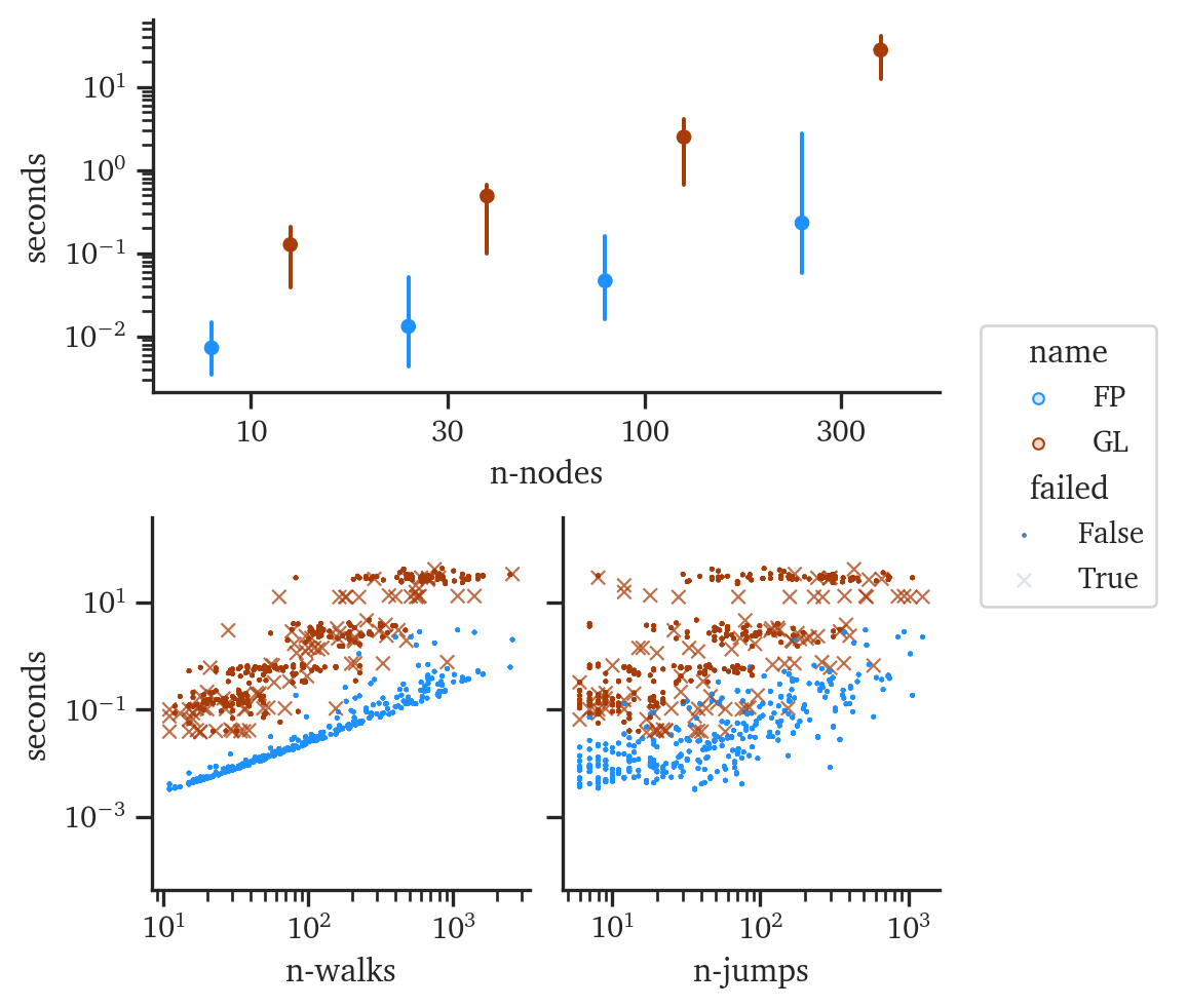
For both Forest Pursuit and GLASSO, runtime efficiency is critical if these algorithms are going to be adopted by analysts for backboning and recovery. Figure 6.7 shows the (log-)seconds against the same parameters from before. For similar sized networks, FP is consistently taking 10-100x less time to reach a result than GLASSO does. Additionally, many of the experiments led to ill-conditioned matrices that failed to converge for GLASSO under any of the regularization parameters tests (the “x” markers in Figure 6.7). As expected, the number of observations plot shows a clear limit in terms of controlling the lower-bound of FPs runtime, since in this serial version every observation runs one more call to MST. On the other hand, GLASSO appears to have significant banding for walk length and observation counts, likely indicating dominance of network size for its runtime.

Figure 6.7: Runtime Scaling (Forest-Pursuit vs GLASSO)

To control for each of the variables, and to empirically validate the theoretical analysis in Approximate Complexity}, a regression of the same three (log-)parametwers was performed against (log-)seconds. The slopes in Figure 6.8, which are plotted on a log-log scale, correspond roughly to polynomial powers in linear scale. In regression terms, we are fitting the log of \[y_{\text{sec}} = ax_{\text{param}}^\gamma\] so that the slope in a log-log plot is $\gamma$.

Figure 6.8: Partial Residuals (regression on computation time)

In a very close match to our previous analysis, the scaling of FP is almost entirely explained by the observation count and random-walk length, alone: the coefficient on network size shows constant-time scaling. Similarly, the scaling with observation count is very nearly linear time, as predicted. The residuals show non-linear behavior for the random-walk length parameter, which would make sense, due to the theoretical $\|E\|\log\|V\|$ scaling of Kruskal’s algorithm. At this scale, $n\log n$ and $n^2\log n$ complexity might appear smaller than linear time, due to the log factor. GLASSO hardly scales with random walk length, and only marginally with observation count. In typical GLASSO, the observation count has already been collapsed to calculate the empirical covariance matrix, so its effects here might be due instead to the cross-validation and the need to calculate empirical covariance for observation subsets. The big difference, however, is GLASSO scaling in significantly superlinear time—almost $O(n^2)$. This is usually the limiting factor for analyst use of such an algorithm in network analysis more generally.