Modifications & Extensions
“Sure, we could include all the of variables in the analysis, but do-calculus (or similar) will usually tell us that we don’t have to.”
– Richard McElreath
Forest Pursuit is a flexible base for adding or modifying behavior as needed. In this chapter we demonstrate two ways to extend it, along with a probabilistic model to serve as a foundation for future extensions. First, we address the perceived shortcoming of FP compared to GLASSO in terms of APS score, showing that a simple modification to the way FP weights edge probability recovers the same performance as GLASSO (at the cost of other scores). Then we use the implicit causal dependency tree structure of each observation, together with the Matrix Forest Theorem [1], [2] to more generally define our generative node activation model. This leads to a generative model for binary activation data as rooted random spanning forests on the underlying dependency graph. Finally, we use this model to continue where FP left off by alternating between estimation of \(R\) an \(B\), in a method we call Expected Forest Maximization (EFM). EFM shows small but consistent improvement in performance over FP, at the cost of computation (and unknown convergence) time.
[2]
O. Knill, “Counting rooted forests in a network,” arXiv, arXiv:1307.3810, Jul. 2013. doi: 10.48550/arXiv.1307.3810.
Forest Pursuit Interaction Probability
Without using stability selection[3], GLASSO is not directly estimating the “support” of the edge matrix, but the strength of each edge. to do similar with FP, we could directly estimate the frequency of edge occurrence using \(R(i,e)\) marginal averages, rather than conditioning on co-occurrence. Simply multiplying each FP edge probability by the co-occurrence probability of each node-node pair gives this as well, which we call FPi: the direct “interaction probability” for each pair of nodes.
[3]
N. Meinshausen and P. Bühlmann, “Stability selection,” Journal of the Royal Statistical Society Series B: Statistical Methodology, vol. 72, no. 4, pp. 417–473, Aug. 2010, doi: 10.1111/j.1467-9868.2010.00740.x.
Simulation Study Revisited
By doing this simple re-weighting, FPi actually beats GLASSO’s median APS for the dataset, but at the cost of MCC and F-M scores (which both drop to between FP and GLASSO), as Figure 7.1 demonstrates. Similarly, the individual breakdown by graph kind in Table 7.1 shows a similar pattern, with FPi coming close to GLASSO for scale-free networks, but exceeding it for trees and matching for block graphs. Still, the difference is small enough, and at such a significant penaly to MCC and F-M scores over a variety of thresholds, that it is hard to recommend the FPi re-weighting unless rate-based edge analysis is desired, e.g. if Poisson or Exponential occurrence models are desired.

Consistent with the increased APS, however, we also see an improvement in MCC-min and MCC-max. If there is a domain-driven reason to select specific thresholds, or if GLASSO is known to provide reasonable results for a given problem, FPi stands a good chance of improving on the optimal or min-connected MCC score.
Simulation Case Study
To illustrate what is going on, we have selected two specific experiments as a case study, in Figure 7.2. In the first, BL-N030S01, a 30-node block graph with 53 random walk samples, has FP performing worse than GLASSO and Ochiai, in terms of APS (which is reported in the legends). We see that FP shows high precision, which drops off significantly to increase recall at all. Only a few edges had high probability (which is usually desirable for sparse approximation), and some of the true edges were missed this way. However, FPi rescaling makes rarer edges fall off earlier in the thresholding, letting the recall rise by dropping rare edges, rather than simply the low-confidence ones.
In the second, SC-N300S01 is a 300-node scale-free network with 281 walks. Both FP and FPi show significantly better recovery capability, since enough walks have visited a variety of nodes to give FP better edge coverage. In this graph, no algorithm comes within 0.25 of FP’s impressive 0.88 APS, especially with 300 nodes and fewer than that many walks.

Generative Model for Correlated Binary Data
Generating multivariate, correlated binary data is of interest across many of the fields discussed in this work, since such models can be used as foundations structural inference (especially if they have a defined likelihood function). One of the foundational generative models for correlated binary data makes direct use of the multivariate-normal’s precision matrix buy sampling directly from it and thresholding values to be binary [4]. In a related sense, the multivariate probit (MVP) is used to analyse such data, treating the likelihood of observed binary outcomes as probabilities from the cumulative distribution function of the underlying multivariate normal.
[5]
H. C. Nguyen, R. Zecchina, and J. Berg, “Inverse statistical problems: From the inverse ising problem to data science,” Advances in Physics, vol. 66, no. 3, pp. 197–261, Jun. 2017, doi: 10.1080/00018732.2017.1341604.
[6]
A. Vasilyev, S. Maier, and R. W. Seifert, “Assortment optimization given basket shopping behavior using the ising model,” Feb. 2025, doi: 10.48550/ARXIV.2502.16260.
Another generative model is the Ising Model, which has long been used as a tool for modeling particle spins in lattice structures, but in the inverse setting is seeing increased application in data science for recovering network structure [5] While techniques like Gibbs sampling might be used to sample from the Ising distribution, a common technique to estimate the structure of the lattice is to perform logistic regression on each node’s activation values using the activation of all other nodes. The equivalence of this Multivariate Logit (MVL) to the Ising model is discussed in [6]
As was briefly mentioned in Roads to Network Recovery, another class of models makes use of the bipartite structures implied by the binary activation data. These degree sequence methods can synthesize other bipartite structures (and therefore, generate binary observations) that match a desired degree distribution [7], [8]. If the case that the true number of nodes is unknown (or should be approximately inferred), a class of models known as the Indian Buffet Process [9] is s distribution over all binary matrices with a finite number of rows. It can therefore sample entire datasets, like the degree sequence models, but with more flexibility in inferring the number of necessary nodes.
[7]
K. Godard and Z. P. Neal, “Fastball: A fast algorithm to randomly sample bipartite graphs with fixed degree sequences,” Journal of Complex Networks, vol. 10, no. 6, Oct. 2022, doi: 10.1093/comnet/cnac049.
[8]
Z. P. Neal, “Randomly sampling bipartite networks with fixed degree sequences,” May 2023, doi: 10.48550/ARXIV.2305.04937.
[9]
T. L. Griffiths and Z. Ghahramani, “The indian buffet process: An introduction and review,” J. Mach. Learn. Res., vol. 12, no. null, pp. 1185–1224, Jul. 2011.
For all of these generative models, there is a lack of model that takes into account the underlying information available to us when we know that the activation structures arise from a spreading process (like random walk visits). Here we propose a compound distribution with a reasonable likelihood that can not only model and generate correlated binary outcomes, but also be inferred using the techniques first discussed for Forest Pursuit. We accomplish this by exploiting the isometry between distributions over random spanning forests and spanning tree distributions over an augmented graph. We are able to derive a simple likelihood and a rapid inference scheme using the Matrix Forest Theorem of Chebotarev and Shamis [1]
Marked Random Spanning Forest (RSFm) distribution
Every spanning forest on a graph described by \(Q\) can be thought of as an equivalent spanning tree over a graph augmented with an extra “source” node, which is connected to every other node with a weight \(\tfrac{1}{\beta}\). Sampling random spanning trees on the augmented graph is equivalent to random spanning forests on the original.[10] We can use this fact to create a distribution for node activation sets based on co-occurrence on a rooted tree.
[10]
K. Avrachenkov, P. Chebotarev, and A. Mishenin, “Semi-supervised learning with regularized laplacian,” Optimization Methods and Software, vol. 32, no. 2, pp. 222–236, Mar. 2017, doi: 10.1080/10556788.2016.1193176.
A “rooted tree” is a tree with a marked node. In Figure 7.3 we see this illustrated, where a randomly sampled tree on the graph augmented with R leads to many subtrees in the original graph. Marking one node (d) at random selects the tree that contains (d,h,e), which corresponds to record \(x_1\) back in Figure 5.2 (a).

Note that the marked node does not necessarily need to be the one that the source “injected” to, since the observed activations set is equivalent for any of (d,h,e) being marked. This is an important symmetry when we will not know which node “actually” started each cascade, during inference.
It means that the node activation set and the graph structure are conditionally independent, given a sampled spanning tree on the augmented graph. Sampling efficiently from a spanning tree distribution is a well studied problem, and we can use that efficiency in combination with a node-marking (categorical) distribution to formulate an overall distribution for node activation.
Therefore, RSFm distribution models the probability of emitting node \(j\) in the \(i\)-th observation as the probability of occurring in the same tree as a marked “root” node \(\phi_{ij}\), given a graph of \(z_E\) edges and a source “distance” parameter \(\beta\). Since the graph is assumed to be independent of the trees sampled on it, we can use the law of total (conditional) probability:
\[
P(x_{ij}|z_E, \phi_{ij}) = \sum_{T\in\mathcal{T}_{+R}}P(x_{ij}| T,\phi_{ij}) P(T|z_E)
\]
Incredibly, the probabilities for \(P(T|z_E)\) and \(P(x|T,\phi)\) all have closed form representations. The spanning tree distribution discussed elsewhere[11], [12] can be used to motivate a spanning forest distribution, which is based on the Laplacian of the augmented graph \(L_+\).1 This means that the probability of a spanning tree in the augmented graph is proportional to the probability of a forest in the original, or, \(P(T\in\mathcal{T}_{+R}|z_E) \propto P(F\in\mathcal{F}|z_E)\).
[12]
R. Zmigrod, T. Vieira, and R. Cotterell, “Efficient computation of expectations under spanning tree distributions,” Transactions of the Association for Computational Linguistics, vol. 9, pp. 675–690, Jul. 2021, doi: 10.1162/tacl_a_00391.
1 Here, \(L_+(G)\) and \(L_+(G/e)\) represent the Laplacian of \(G_{+R}\) and \(G_{+R}\) without edge \(e\), respectively.
\[ P(x_{ij}|z_E, \phi_{ij}) = \sum_{F\in\mathcal{F}}P(x_{ij}| F,\phi_{ij}) P(F|z_E) \]
Using this equivalence on Kirchoff’s matrix tree theorem gives the Chebotarev-Shamis Forest Theorem[1] for the partition function over spanning forests \(Z_\mathcal{F}\), which gives a closed form for Equation 5.2 over all spanning forests (not just spanning trees on a subgraph). If \(\mu(F)\) is a measure on forests, e.g. the product of weights of edges, then:
[1]
P. Chebotarev and E. Shamis, “The matrix-forest theorem and measuring relations in small social groups,” arXiv, arXiv:math/0602070, Feb. 2006. doi: 10.48550/arXiv.math/0602070.
\[ \begin{gathered} P(F|z_E) = \frac{1}{Z_\mathcal{F}} \mu(F)\\ Z_\mathcal{F} = \det{(I+\beta L)} \end{gathered} \]
There are a variety of techniques already cited for sampling from this distribution, because of the connection with spanning trees on an augmented graph. This means we can sample from RSFm with only one modification from normal spanning tree distributions:
- Generate random spanning trees on \(G_{+R}\), according to \(P(F|z_E)\).
- Uniformly sample a marked node \(\phi\).
- Activate all nodes connected to \(\phi\) in the induced spanning forest.
To do inference, however, we may again use the forest kernel \(Q\), which gives us probabilities for node co-occurrence on trees in a spanning forest. We only need to combine entries of Q for the observed nodes to determine the likelihood of an observation. \(\sum_\mathcal{F} P(x_{ij}|F,\phi_{ij})\) would be the probability of a node occurring (or not) on the same subtree as the marked node, and as previously discussed, this is just \(Q(u\in V_i,\phi)\) for each node that is activated, and \(1-Q(v\notin V_i,\phi)\), for each that is not. Note that this assumes we marginalize over a uniformly distributed \(\phi\).
Model Specification
The overall model that fills out the gaps left in Equation 5.5 has the form:
\[ \begin{aligned} \pi_{e\in E} &\sim \operatorname{Beta}_E(\alpha, 1-\alpha) \\ z_{e\in E} &\sim \operatorname{Bernoulli}_E(\pi_e) \\ \phi_{i\in I, j\in J} &\sim \operatorname{Categorical}_I(\theta) \\ x_{i\in I,j\in J} &\sim \operatorname{RSFm}_K(\beta, z_e, \phi_n) \\ \end{aligned} \]
The above still has the problem of needing an estimate for \(Q=(I+\beta L_z)\) based on the graph described by the active edges in \(z\). It could be done with a monte-carlo sampler, though the nested likelihood may prove difficult.
The conditional independence mentioned previously could lend itself to a collapsed Gibbs-sampling scheme. Each observation is a marked node and a sampled random spanning forest, which can equivalently be described as a sampled spanning tree over the activated nodes, like originally discussed in Equation 5.2. This works because we can marginalize out the equal marked-node probability \(\phi\) if we assume a uniform probability of selection for each node, and because we can jointly use the desire-path model to derive an estimate for z_E from the internal edge samples of RSFm.
Beginning with the FP point estimate, each edge in every spanning subtree can be efficiently resampled according to the Bayesian Spanning Tree distribution from [11]. Once every edge in a tree has been resampled, the overall estimate for the desire path network can be updated, and sampling can continue. This would be very similar to the way collapsed Gibbs sampling works for Latent Dirichlet Allocation[13], but with edges selected from a spanning forest distribution instead of “topics” from a multinomial. Derivations and implementation of such a scheme is left for future work.
[11]
L. L. Duan and D. B. Dunson, “Bayesian spanning tree: Estimating the backbone of the dependence graph,” arXiv, arXiv:2106.16120, Jun. 2021. doi: 10.48550/arXiv.2106.16120.
[13]
D. M. Blei, A. Y. Ng, and M. I. Jordan, “Latent dirichlet allocation,” Journal of machine Learning research, vol. 3, no. Jan, pp. 993–1022, 2003, doi: 10.7551/mitpress/1120.003.0082.
Expected Forest Maximization
Another possibility is to approach the problem as a kind of matrix factorization, jointly estimating \(B\) and \(R\) in an alternating manner. Where Forest Pursuit was an empirical Bayes estimate for \(R\), alternating from there between \(B\) and \(R\) leads to a simple Expectation Maximization scheme.
Factorization & Dictionary Learning
Jointly finding a sparse representation of data using a linear combination of basis vectors (called a “dictionary”), and finding an optimal dictionary with which to do the embedding, is called “sparse dictionary learning”. One of the original proposed methods to solve this was the Method of Optimal Directions (MOD)[14], which uses a sparse “pursuit”-like method to find the representation vectors, and then uses that representation to find \(\hat{B}\gets XR^+\).2 However, our desire path estimation for independent (arcsine) Bernoulli edges gives an efficient workaround to needing the pseudo-inverse. Based on our interpretation of the forest kernel, counting co-occurrences on trees is equivalent to estimating the inverse of the regularized graph laplacian, anyway. Each Forest Pursuit estimate can yield a new distance \(d_Q(u,v)\), which can be used as a regularized shortest-path distance for small enough \(\beta\). Then, new steiner tree estimates will approximate the modes of each spanning tree distribution, which can be used for a new desire-path estimate of the edges, and so-on.
[14]
K. Engan, S. O. Aase, and J. Hakon Husoy, “Method of optimal directions for frame design,” in 1999 IEEE international conference on acoustics, speech, and signal processing. Proceedings. ICASSP99 (cat. no.99CH36258), IEEE, 1999. doi: 10.1109/icassp.1999.760624.
2 \(R^+\) is the pseudo-inverse of \(R\).
Probabilistically, we are finding the expectation over spanning forests (collapsing over uniform \(\phi\)) in the form of calculating \(Q\), and then maximizing the likelihood of each observation through Forest Pursuit. The proposed algorithm Expected Forest Maximization is outlined in Algorithm 1.
\begin{algorithm} \caption{Expected Forest Maximization (EFM)} \begin{algorithmic} \Require $X\in \mathbb{B}^{m\times n}, d_K\in \mathbb{R}_{\geq 0}^{n\times n}, 0<\alpha<1$ \Ensure $R \in \mathbb{B}^{m \times {n\choose 2}}$ \Procedure{EFM}{$X, d_K, \alpha, \beta, \epsilon$} \State $R \gets $\Call{ForestPursuit}{$X, d_K$} \State $\hat{\alpha}_m\gets$\Call{DesirePathBeta}{$X,R, \alpha$} \While {$\|\hat{\alpha}-\alpha\|_{\infty}>\epsilon$} \State $\alpha_m \gets \hat{\alpha}_m$ \State $Q \gets (I+\beta L_{\text{sym}}(\alpha_m))^{-1}$ \State $d_K \gets d_Q$ \State $R \gets $\Call{ForestPursuit}{$X, d_K$} \State $\hat{\alpha}_m\gets$\Call{DesirePathBeta}{$X,R, \alpha_m$} \EndWhile \State \textbf{return} $\hat{\alpha}_m$ \EndProcedure \end{algorithmic} \end{algorithm}
In practice, we limit iterations to less than 100, though that limit is not reached in our testing. We use a small \(\beta=10^{-3}\) to approximate shortest path distances, and we can do so within the forest pursuit loop to avoid inverting large matrices. Instead of \(d_K\), the graph structure itself (once an initial estimate is made) can be passed to Forest Pursuit, where each subgraph can estimate \(d_{Ki}\) independently. After all, shortest paths in a subgraph when we assume no hidden nodes will be the same as in the global graph. Note as well the use of the symmetric normalized Laplacian \(L_{\text{sym}}\). We use this to enable the splitting of inversions like this, because the global Laplacian has higher possible degrees than the subgraph, and we do not wish to bias Steiner tree estimation by node degree. Not doing so leads to rapid divergence of the loss function, as all MSTs will tend toward star-graphs around the highest-degree node.
EFM Simulation Study
One-shot Forest Pursuit appears to perform quite well, so it’s useful to quantify the expected gain in performance by repeating it an unknown number of times. There are no generic guarantees for EM convergence, though anecdotally the number of iterations was limited in our experiments to under a thousand, and that limit was never hit while using a covergence parameter of \(\epsilon=1\mathrm{e}-5\).
The distribution of E[MCC] score change vs. FP is shown in Figure 7.4.

While useful, it’s not clear whether individual edges are more likely to be “true” edges, given a bigger change in EFM score. To test this, a logistic regression was performed for every experiment in MENDR against the true edge values, using the change in scores on those edges between FP and EFM as training data. To avoid overfitting, a significant amount of regularization was applied, chosen using 5-fold crossvalidation. The coefficients for all experiments are shown as a histogram in Figure 7.5.

The graph kind did not make a significant difference to EFM improvement, but overall log-odds improvement is very low.Still, the value is positive accross the entire dataset, so EFM does have a very small-but-nonzero impact on improving edge prediction.
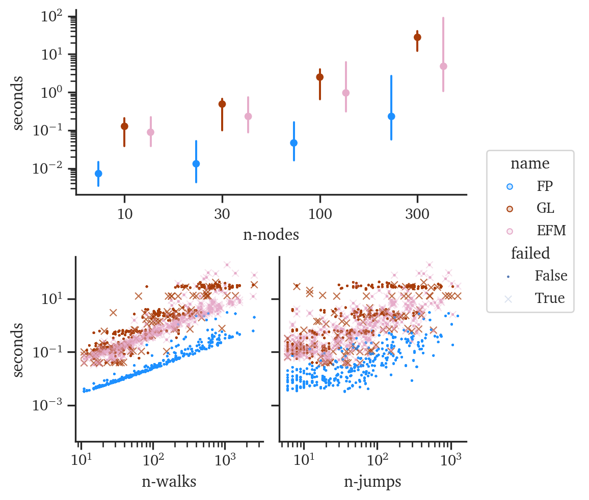
The runtime graphs can also be updated, with EFM shown in Figure 7.6 and Figure 7.7 against FP and Glasso. EFM still ran significantly faster than GLASSO in this region. However, the scaling with network size is no longer constant-time, especially since convergence used above is the max-abs error, which requires that every node reach a minimum level of convergence and might take much longer, overall.